Z-score

What is a Z-score?

Test Score Example

Without a formal definition, it tells you how you are relative to everyone else. Let's begin with an example. Say you are in a class of 10 students and took a biology test. These were the scores: 86, 92, 81, 86, 87, 94, 97, 85, 93, 88. Let's say you got the 92. That is a pretty good score. But how do we tell how well you did from everyone else? The values given outright are called the raw values. Think of these, original numbers, or raw numbers, as a perspective of how you can see the numbers. What if I told you, we could see it another way? Here come the z-scores. We do need to know two other pieces of information: the mean and the standard deviation.

Calculating Components of Z-Score

First is the mean, or \(\mu\), and the other is the standard deviation, or \(\sigma\), of the population, i.e., in this situation is the classroom. Adding the scores and dividing them by the number of students will get you the mean: (86+92+81+86+87+94+97+85+93+88)/10 = 88.9. With this information alone we understand that you did better than the average. Maybe this would suffice, but let's get a little more detailed. Let's find out the standard deviation, or the spread of the numbers. This will require taking the square root of the average squared difference between the raw value and the mean: \(\sigma = \sqrt{\frac{\Sigma^{N}_{i=1}(x_i - \mu)^2}{N}}\). Since we know that there are 10 students, N = 10. This means we will have the summation of 10 values at the top of the fraction from 1 to 10. \(x_i\) simply means any individual score of a student which is the raw score because it has yet to be converted into the new perspective of z-scores. \(x_1\) = 86 and \(x_2\) = 92 and so on until \(x_{10}\), which is 88. For the first difference squared that is \(x_1\), it is \((x_1-\mu)^2=(86-88.9)^2=8.41\). The total set of ten after the operation is 8.41, 9.61, 62.41, 8.41, 3.61, 26.01, 65.61, 15.21, 16.81, 0.81. Taking the average of that is summing them and dividing by 10 or approximately 21.69. Then the square root of that number will be about 4.66 for the standard deviation.

Calculating Your Z-score

We have \(\mu=88.9\) and \(\sigma=4.66\), so we can use the z-score equation: \(z = \frac{x-\mu}{\sigma}\). The \(x\) is any raw value that can be converted to a z-score, so our original scores. Now for the moment of truth for your score: \(z = \frac{92-88.9}{4.66}\) which is about 0.67. But, what does this mean? First, we look at the sign. We see that it is positive. Since the sign is positive you are above the mean of the class. If it was negative, you would be below the class mean. Next, the value, 0.67. Notice that the equation is divided by the standard deviation. This means we are based in units of standard deviation. If we have a z-score of 1, we are 1 standard deviation away from the mean in the positive direction, i.e., above the mean. We can have fractions of a standard deviation. This is the case. We have 0.67 of a standard deviation above the mean. For all the z-scores they can be calculated (and rounded) to be the following: -0.62, 0.67, -1.70, -0.62, -0.41, 1.10, 1.74, -0.84, 0.88, -0.19.

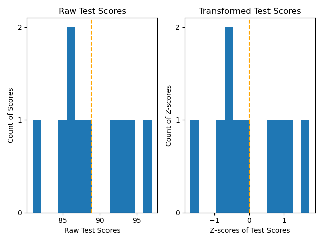
Comparing Raw Values to Z-score Values

To elucidate the relationship, let's sort both the raw test scores and the z-scored version of the test scores in ascending order to compare. The raw values are 81, 85, 86, 86, 87, 88, 92, 93, 94, 97. And the z-score values respectively are -1.70, -0.84, -0.62, -0.62, -0.41, -0.19, 0.67, 0.88, 1.10, 1.74. We now see that with the z-scores, unlike the raw scores go from negative numbers to 0 to positive numbers. Remember with z-scores, the mean of the set has a z-score of 0: \(z = \frac{x-\mu}{\sigma} = \frac{\mu-\mu}{\sigma} = 0\). This is significant because now we gain information of directionality relative to the mean, positive or negative, and by how much with its magnitude. We see that the larger the negative number, the further to the left the number can be from the mean, so it is increasing smaller: -0.41 is to 87 as -1.70 is to 81. On the contrary, the larger the positive number, the further to the right the number can be from the mean, so it is increasing larger: 0.67 is to 92 as 1.74 is to 97. We can plot the histograms of both sets of numbers below with their mean in orange to see the distributions.

Comparison of Uses: Raw vs Z-score

We see from the figure that the distributions are the same with only the numbers associated with them changed. Again, it is perspective. The major difference is that with z-scores we gained some intrinsic information of all the scores baked into the value. Going back to the beginning, if we said you had a score of 92. You may have the best score, the worst score, or average score. We do not know. If we told you, you had a z-score of 0.67, you now know you did better than the average by some. Okay, but let's argue further. Why not just argue that I just need my score and the average score? 92 and 88.9 are the numbers, so you know that you did better than the average just like the z-score. However, you would be missing the standard deviation piece of the information. We know you did better than the average, but we do not know how everyone else did in the distribution. Maybe there was a wide spread of scores. If so, that means there can be many people who did better and worse compared to you. On the other hand, with a smaller spread, this would mean that everyone had similar scores to you. With a z-score, we actually standardized or normalized the spread, so this is a more reliable comparison to know where you are within the distribution of scores. This is if your distribution is normal, you can apply the 68-95-99.7 rule, or look up the area under the curve to find the relative percentile you are from all the other scores. Interpreting further requires knowing if the distribution is normal or not.

Implications of Normal vs Non-Normal Distribution

When we know that the values fall under a normal distribution, we know that 68% percent of the values fall within 1 standard deviation away from the mean. That means on each side is 68%/2 or 34%. So a z-score of 1, would be 34% beyond the middle point which is 50% or 84%, meaning z=1 would mean it contains 84% of all the scores below it. With a z-score of 0.67, it is not so clean cut, and we should use a z-table. We can search online for a z-table, find a z-table with the positive values because we have a positive z-score in our case, and scan down the left most column to find the tenths place of the z-score: 0.6. Then we scan across the top of the table along the columns to find the hundreths place: 0.07. The intersection will find the value: 0.7486 or 74.86% of all the values in our set are below our value.

What if we find out that our distribution is not normal? How would we interpret these z-scores? It can be used to get a rough idea, but note that we would not be able to use the z-table to connect it to a percentile. Instead we can use Chebyshev's theorem to find the minimum proportion of data within k standard deviations of the mean: \(1-\frac{1}{k^2}\) with k>1. This can be used on any distribution, so not just non-normal distributions. So if within 2 standard deviations from the mean, the math simplifies as follows: \(1-\frac{1}{k^2} = 1-\frac{1}{2^2} = 1-\frac{1}{4} =0.75 \). For 3 standard deviations from the mean we have the following: \(1-\frac{1}{k^2} = 1-\frac{1}{3^2} = 1-\frac{1}{9} = 0.8889 \). This means within 2 standard deviations from the mean, there should be at least 75% of the data or scores, and for 3 standard deviations it would be at least 88.89% of the scores (approximately). So with 0.67, it may not be so useful but we know that we are less than 2 standard deviations so we can say it does not contain at least 75%. In other words we contain less than 75% of the scores with our raw value of 92.

Summary

Z-scores is another perspective on a value within a set of values. It has directionality and magnitude of its value relative to the mean. Moreover, it gives an approximate (or more exact with normally distributed numbers) idea of how many values are below or above it relative to all the values. Using a raw value gives you a piece of information, but using a z-score gives you the larger picture. Note that z-scores are so versatile and can be used in medical implications such as bone density, height, and blood pressure. To read more about normal distributions, read this post.

• Read More Posts