Normal Distribution

What is a probability distribution?

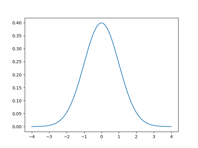
First, a normal distribution is a type of probability distribution, but what is a probability distribution? Imagine a cartesian coordinate system: an x and y axis. The x-axis would be a range of possible values and the y-axis would be the probability that any of these particular values would occur. This means that if the height of the y axis is high, there is a high probability of finding that value of all the x values and vice versa. Now, the figure above shows the shape of what a normal distribution looks like with the center being the value that is most likely to occur. It then falls on both sides outwards towards what are known as the tails, where the graph pinches off on the left and right sides. The left and right tails are the values that are less likely to occur.

Why is this distribution important?

It is a heuristic for sciences to represent an unknown distribution as such. This is because of the Central Limit Theorem. It states that regardless of the distribution, when one takes a sample of the population and plots the mean, and does this repeatedly on a histogram, the distribution will tend towards the shape of a normal distribution! This means that statistical methods used in normal distributions can be used on other distributions as it approaches the normal shape with an increasing number of samples.

How is it described mathematically?

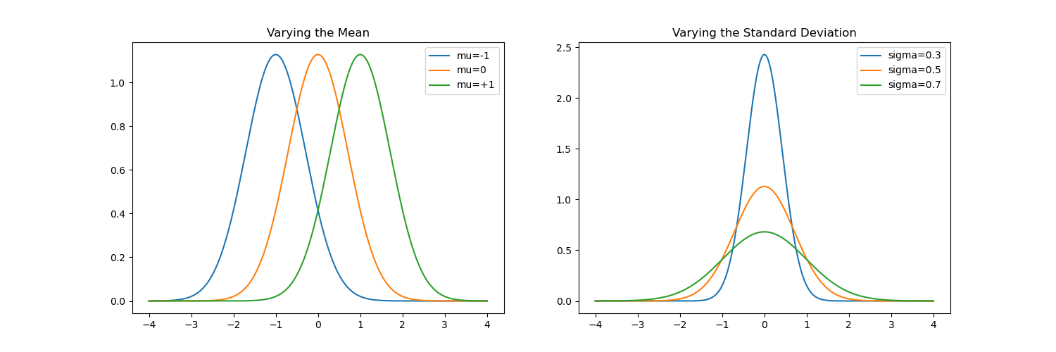
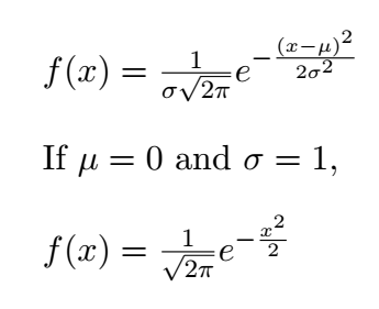
There are two important variables: (1) μ (pronounced mu), the mean and (2) σ (pronounced sigma), the standard deviation. The mean sets the center of the distribution, where the peak is, shifting the whole distribution to the left or the right. The standard deviation describes the spread of the bell curve, with a larger value spreading out the tails further left and right and decreasing the peak of the curve as it preserves it's constant area.

Intuitive Understanding of Standard Deviation

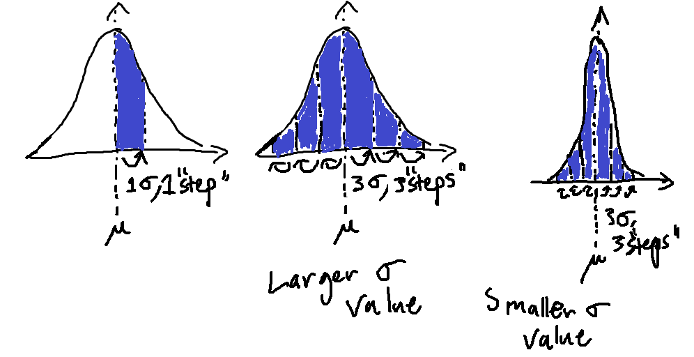
Before, I mentioned that the standard deviation describes the spread, and a way to visualize that is to see a standard deviation as a "step", either to the left or right along the x-axis, away from the mean. Moreover, with that step, a section of the area underneath the curve is covered. Most of the area of the curve is covered between 3 "steps" to the left and 3 "steps" to the right of the mean. So, if the standard deviation is low in value, then it is like 3 small steps from both sides of the mean to cover nearly all the area, meaning less spread. If the standard deviation is high, it is like 3 large steps, making the shape more spread out.

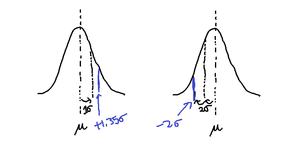
While tracking the distance in "steps" from the mean, it is important to indicate which direction one goes. Steps to the right of the mean are positive, and inversely, steps to the left are negative. For example, an x-value along the x-axis can be +1 standard deviation away, and another x-value can be -2 standard deviations away. If a value is 0 standard deviations away from the mean, the value is at the mean and is the mean. It is also important to know that instead of these whole steps of 1 standard deviation, there can be fractions of one. For example, an x-value can be +1.35 standard deviations from the mean. The term to know where any particular value is along the x-axis by standard deviations away from the mean is called the z-score. Therefore, you could rephrase any of these statements, but to rephrase the prior statement, the z-score of this value is +1.35. To be absolutely clear, standard deviation is a fixed value based on the shape of the distribution, and the z-score just uses that as a basis of measurement for any particular value within that distribution.

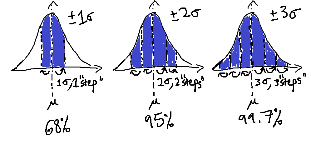
Finally, to quantify how much area is covered with each standard deviation, start visualizing a line down the middle of the peak, and draw another two lines, one to the left and one to the right of it, each equally spaced from the center. If one expands outward and covers 68% of the area underneath the curve, this is known as ±1 standard deviation from the mean, or the area covered between one "step" to the left and one "step" to the right of the mean. Expand further outward to cover 95% of the area, and this is ±2 standard deviations, the area of 2 "steps" on either side. Expand to 99.7% of the area and this is ±3 standard deviations from the mean, the area of 3 "steps" on either side. With more standard deviations, 4, 5, 6, and onwards, it covers more of the remaining area but to much less of an effect.

Characteristics of the normal distribution

The area underneath the curve is equal to 1. Meaning that values underneath the curve can be represented as percentiles. For instance, 0.75 is the 75th percentile, so that would be a value that is above 75% of the values of that distribution. In fact, there is a table called a standard normal table that allows one to look up how much area is covered underneath the curve from the left tail to a particular z-score. This is useful for calculations involving z-scores. Another fact is about the distribution is that the mean, median, and mode are the same value.

How do I use the normal distribution?

In nature, it is common to find many observations in the average range and less on either extremes. Some examples include test scores, height, and so on. However, when someone says they are of a particular score or height, it is not completely telling of how they are relative to everyone else. When everyone has a high score for instance on a test, it may just mean that the test was easier, but if one measures relative to others by how many standard deviations they are from the mean, this becomes more meaningful. This is done by calculating z-scores. To find out more on how, read my z-score post!

• Read More Posts